DBMS

Note - This notes are made from videos of Sanchit Jain Youtube (Knowledge Gate). I will really suggest to watch those videos because he explained all these really well. I can guarantee that you will not get bored at any point.

E-R Diagram
Conversion of E-R diagram into relational model
Basics of relational model & functional dependancy
Idea about keys/types
Normalization (INF-BCNF)
Lossless decomposition & dependancy preserving
Indexing and Physical Structure (B, B+ Tree)
SQL, RA, RC
Transaction
Concurrency Control

Basic Fundamentals

Difference between Data, Information, Database

Data - Raw and Isolated facts about an entity (recorded). eg. text, audio, video, image, map, etc.
Information - Processed, meaningful, usable data
Database - Collection of similar / related data - Database: A database is a collection of related data which represents some aspect of the real world. A database system is designed to be built and populated with data for a certain task.
DBMS - Software used to create, manipulate and delete data - Database Management System (DBMS) is a software for storing and retrieving users’ data while considering appropriate security measures. It consists of a group of programs which manipulate the database. The DBMS accepts the request for data from an application and instructs the operating system to provide the specific data. In large systems, a DBMS helps users and other third-party software to store and retrieve data.

Database management systems were developed to handle the following difficulties of typical File-processing systems supported by conventional operating systems.

Data redundancy and inconsistency
Difficulty in accessing data
Data isolation – multiple files and formats
Integrity problems
Atomicity of updates
Concurrent access by multiple users
Security problems

Disadvantage of File System

Data Redundancy - Data redundancy occurs when the same piece of data exists in multiple places
Data Inconsistency - Data inconsistency is when the same data exists in different formats in multiple tables
Difficulty in Accessing Data
Data Isolation - This problem arises due to the scattering of data in various files with various formats.
Integrity Problem - Data integrity is the maintenance of, and the assurance of, data accuracy and consistency over its entire life-cycle and is a critical aspect to the design, implementation, and usage of any system that stores, processes, or retrieves data
Atomicity of Updates - Atomicity is a feature of databases systems dictating where a transaction must be all-or-nothing. That is, the transaction must either fully happen, or not happen at all. It must not complete partially.
Concurrent Access Anomalies - Anomalies occur when changes made by one user gets lost because of changes made by other user.
Security Problem - Read, Edit, View etc

OLAP VS OLTP

	Online Analytical Processing	Online Transaction Processing
type	Historical Data	Current Data
purpose	Subject Oriented	Application Oriented
use	decision making	day to day operations
Size	TB, PB	MB, GB
who	CEO MD GM	clerks, managers
Operations	Read	Read/Write

1. Entity Relationship Diagram

Introduction and Basics
Entity and Entity Set
Attributes and types
Relationship
Strong and weak Entity Set
Traps
Conversion

Introduction and Basics

Introduced by Dr. Peter Chen in 1976
A non-technical design method works on conceptual level based on the perception of real world
Consists of Collection of basic objects called entities and of relationship among there objects and attributes which defines their properties.
Free from ambiguties and provides a standard and logical way of visualizing data
Basically it is a diagrammatic representation easy to understand even by non-technical user.

ER diagram or Entity Relationship diagram is a conceptual model that gives the graphical representation of the logical structure of the database.
It shows all the constraints and relationships that exist among the different components.
An ER diagram is mainly composed of following three components- Entity Sets, Attributes and Relationship Set.

Student ER

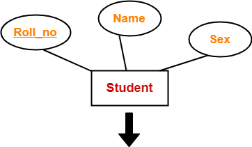
Roll_no is a primary key that can identify each entity uniquely.
Thus, by using a student’s roll number, a student can be identified uniquely.

Entity Relationship Model

Entity, Entity Sets and its types

Entity - An entity is a thing or an object in the real world that is distinguishable from other objects based on the values of the attributes it possess.
Types of Entities :-
- Tangible: Entities which physically exist in real world eg. Car, Pen, BankLocker
- Intangible: Entities which exists logically eg. Account
Entity Sets - Collection/Set of same types of entities ie. that show same properties or attributes called entity set.
1. Strong Entity Set:
- A strong entity set is an entity set that contains sufficient attributes to uniquely identify all its entities.
- In other words, a primary key exists for a strong entity set.
- Primary key of a strong entity set is represented by underlining it.
1. Weak Entity Set:
- A weak entity set is an entity set that does not contain sufficient attributes to uniquely identify its entities.
- In other words, a primary key does not exist for a weak entity set.
- However, it contains a partial key called a discriminator.
- Discriminator can identify a group of entities from the entity set.
- Discriminator is represented by underlining with a dashed line.

ER Diagram and Relationship Model

ER diagram	Relational Model
1. Entity can not be represented in an ER diagram as it is instance/data	1. Entity can be represented in an relational model by row/tuple/record
2. Entity set is represented by rectangle in ER diagram.	2. Entity set in represnted by table in relational model.

Attributes

Attributes - Attributes are the descriptive properties which are owned by each entity of an Entity Set.

For each attribute there is a set of permitted values called domains (ex- roll no should be numeric).
In ER diagram represented by ellipse or oval, while in relational model by a separate column.

Types of Attributes

Sr. No.	Simple-Composite	Single-Multivalued	Stored-Derived
1.	Simple cannot be divided further, represented by simple oval	Single can have only one value at a instance of time (eg. college ID)	Stored how value is stored in the data base, represented by simple oval
2.	Composite can not be divided further simple attributes, represented by oval connected to a oval	Multivalued can have more than one value at a instance of time (eg. Email), represented by double oval, need to create separate table with primary key	Derived how value can be computed in run time using stored attribute, represented by dotted attribute (age calculated from dob)

Simple Attributes - Simple attributes are those attributes which cannot be divided further. Ex. Age
Composite Attributes - Composite attributes are those attributes which are composed of many other simple attributes. Ex. Name, Address
Multi Valued Attributes - Multi valued attributes are those attributes which can take more than one value for a given entity from an entity set. Ex. Mobile No, Email ID
Derived Attributes - Derived attributes are those attributes which can be derived from other attribute(s). Ex. Age can be derived from DOB.
Key Attributes - Key attributes are those attributes which can identify an entity uniquely in an entity set. Ex. Roll No.

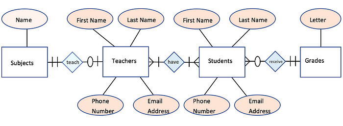
Relationship in a ER Diagram

Relationship - is an association between two or more entities of same or different entity set.

No representation in ER diagram as it is an instance or data.
In relational model represented either using a row in a table.

Relationship type/set - A set of similar type of relationship

In ER diagram represented by a diamond
In relational model either by a separate table or by separate column (foreign key)
Every relationship type has three components
- Name
- Degree
- Cardinality ratio/Participation Constraints

Degree of a relationship in a ER diagram

Degree of a Relationship Set - means the number of entity set associated (participated) in the relationship set.
Most of relationship sets in the ER diagram are binary. Occasionally however relationship sets involve more than two entity sets.
eg. Binary, Ternary, Quaternary, N-ary
Unary Relationship Set - Unary relationship set is a relationship set where only one entity set participates in a relationship set.
Binary Relationship Set - Binary relationship set is a relationship set where two entity sets participate in a relationship set.
Ternary Relationship Set - Ternary relationship set is a relationship set where three entity sets participate in a relationship set.
N-ary Relationship Set - N-ary relationship set is a relationship set where ‘n’ entity sets participate in a relationship set.

Cardinality Ratio and Mapping Cardinalities

Cardinality constraint defines the maximum number of relationship instances in which an entity can participate.
can be used in decscribing relationship set of any degree but is most useful in binary relationship.
Mapping Cardinalities
- One to One
- One to Many
- Many to One
- Many to Many

Every one to one relationship is also a one to many and many to one, many to many relationship

One-to-One Cardinality - An entity in set A can be associated with at most one entity in set B. An entity in set B can be associated with at most one entity in set A.
One-to-Many Cardinality - An entity in set A can be associated with any number (zero or more) of entities in set B. An entity in set B can be associated with at most one entity in set A.
Many-to-One Cardinality - An entity in set A can be associated with at most one entity in set B. An entity in set B can be associated with any number of entities in set A.
Many-to-Many Cardinality - An entity in set A can be associated with any number (zero or more) of entities in set B. An entity in set B can be associated with any number (zero or more) of entities in set A.

Constraints:

Relational constraints are the restrictions imposed on the database contents and operations. They ensure the correctness of data in the database.

Domain Constraint - Domain constraint defines the domain or set of values for an attribute. It specifies that the value taken by the attribute must be the atomic value from its domain.
Tuple Uniqueness Constraint - Tuple Uniqueness constraint specifies that all the tuples must be necessarily unique in any relation.
Key Constraint - All the values of the primary key must be unique. The value of the primary key must not be null.
Entity Integrity Constraint - Entity integrity constraint specifies that no attribute of primary key contain a null value in any relation.
Referential Integrity Constraint - It specifies that all the values taken by the foreign key must either be available in the relation of the primary key or be null.

Keys:

A key in DBMS is an attribute or a set of attributes that help to uniquely identify a tuple (or row) in a relation (or table). Keys are also used to establish relationships between the different tables and columns of a relational database. Individual values in a key are called key values.

Types of Keys:

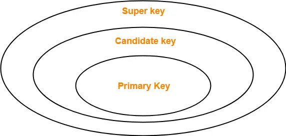
Super-Key-Candidate-Key-Primary-Key

Super Key - A superkey is a set of attributes that can identify each tuple uniquely in the given relation. A super key may consist of any number of attributes. This means that all those columns of a table than capable of identifying the other columns of that table uniquely will all be considered super keys. Super Key is the superset of a candidate key.
Candidate Key - A set of minimal attribute(s) that can identify each tuple uniquely in the given relation is called a candidate key. The Primary Key of a table is selected from one of the candidate keys. So, candidate keys have the same properties as the primary keys. There can be more than one candidate keys in a table.
Primary Key - A primary key is a candidate key that the database designer selects while designing the database. Primary Keys are unique and NOT NULL.There can be only one primary Key in a table. Also, the primary Key cannot have the same values repeating for any row. Every value of the primary key has to be different with no repetitions. Any value in the primary key cannot be changed by any foreign keys which refer to it.
Alternate Key - Candidate keys that are left unimplemented or unused after implementing the primary key are called as alternate keys.
Foreign Key - An attribute ‘X’ is called as a foreign key to some other attribute ‘Y’ when its values are dependent on the values of attribute ‘Y’. The relation in which attribute ‘Y’ is present is called as the referenced relation. The relation in which attribute ‘X’ is present is called as the referencing relation.
Composite Key - A primary key composed of multiple attributes and not just a single attribute is called a composite key.
Unique Key - It is unique for all the records of the table. Once assigned, its value cannot be changed i.e. it is non-updatable. It may have a NULL value.

Participation Constraints

Participation Constraints

Specifies weather the existance of an entity depends on its being related to another entity via a relationship type
these constraints specify the minimum and maximum number of relationship instance that each entity can/must participates in.

Max Cardinality

It defines the maximum number of times on entity occurence participating in a relationship.

Min Cardinality

It defines the minimum number of times on entity occurence participating in a relationship.

Types of Participation

Partial Participation - Not all entities are involved in the relationship. Partial participation is represented by single lines.
Total Participation - Each entity is involved in the relationship. Total participation is represented by double lines.

3. Functional Dependency

Functional Dependencies
Normalization
Indexing, Physical Structures
Transaction

Functional Dependencies

Functional Dependencies
The functional dependency is a relationship that exists between two attributes. It typically exists between the primary key and non-key attribute within a table.
In any relation, a functional dependency α → β holds if- Two tuples having same value of attribute α also have same value for attribute β.
The left side of FD is known as a determinant, the right side of the production is known as a dependent.

Types of Functional dependency

Trivial Functional Dependencies –
- A functional dependency X → Y is said to be trivial if and only if Y ⊆ X.
- Thus, if RHS of a functional dependency is a subset of LHS, then it is called a trivial functional dependency.
Non-Trivial Functional Dependencies –
- A functional dependency X → Y is said to be non-trivial if and only if Y ⊄ X.
- Thus, if there exists at least one attribute in the RHS of a functional dependency that is not a part of LHS, then it is called a non-trivial functional dependency.
- When X ∩ Y is NULL, then X → Y is called as complete non-trivial.

Closure of Attribute Set

Closure of an attribute set A can be defined as a set of attribute which can be functionally determined from it denoted by F^+.
The set of all those attributes which can be functionally determined from an attribute set is called a closure of that attribute set.

Armstrong’s Axiom/Rule

Armstrong axioms holds on every relational database can be used to generate closure set

Primary Rules (RAT)

Reflexivity : if X ⊆ Y, then X -> Y
Augmentation : if X -> Y, then XZ -> YZ
Transitivity : if X -> Y && Y -> Z, then X -> Z

Secondary Rules

Union : if X -> Y && X -> Z, then X -> YZ
Decomposition : if X -> YZ, then X -> Y && X -> Z
Pseudo_Transitivity : if X -> Y && WY -> Z, then WX -> Z
Composition : if X -> Y && Z -> W, then XZ -> YW

Equivalency of Functional Dependency

Two or more than two sets of functional dependencies are called equivalence if the right-hand side of one set of functional dependency can be determined using the second FD set, similarly the right-hand side of the second FD set can be determined using the first FD set.

Canonical Cover, Minimal Set, Irreducible set of FD

A canonical cover or irreducible a set of functional dependencies FD is a simplified set of FD that has a similar closure as the original set FD.

6. Decomposition of a Relation:

The process of breaking up or dividing a single relation into two or more sub relations is called the decomposition of a relation.

Properties of Decomposition:

Lossless Decomposition - Lossless decomposition ensures
- No information is lost from the original relation during decomposition.
- When the sub relations are joined back, the same relation is obtained that was decomposed.
- If a relation R is decomposed into two relative R1 R2 then it will be loss-less iff
1. attr(R1) ∪ attr(R2) = attr(R)
2. attr(R1) ∩ attr(R2) ≠ Φ
3. attr(R1) ∩ attr(R2) -> attr(R1) or attr(R1) ∩ attr(R2) -> attr(R2)
Dependency Preservation - Dependency preservation ensures
- None of the functional dependencies that hold on the original relation are lost.
- The sub relations still hold or satisfy the functional dependencies of the original relation.
- If a table R having FD set F, is decomposed into two tables R1 and R2 having FD set F1 and F2 then F1 ⊆ F⁺ F2 ⊆ F⁺ (F1 ∪ F2)⁺ = F⁺

Types of Decomposition:

Lossless Join Decomposition:
- Consider there is a relation R which is decomposed into sub relations R1, R2, …., Rn.
- This decomposition is called lossless join decomposition when the join of the sub relations results in the same relation R that was decomposed.
- For lossless join decomposition, we always have- R1 ⋈ R2 ⋈ R3 ……. ⋈ Rn = R where ⋈ is a natural join operator
Lossy Join Decomposition:
- Consider there is a relation R which is decomposed into sub relations R1, R2, …., Rn.
- This decomposition is called lossy join decomposition when the join of the sub relations does not result in the same relation R that was decomposed.
- For lossy join decomposition, we always have- R1 ⋈ R2 ⋈ R3 ……. ⋈ Rn ⊃ R where ⋈ is a natural join operator

5. Normalization

Why need of Normalization

Idea
- In the table student info we have tried to store entire data about student.
Result
- Entire branch data of a branch must be repeated for every student of the branch
Disadvantages
1. Insertion, Deletion and Modification Anomalies
2. Inconsitency (data)
3. Increase in database size and increase in time (slow)
Insertion anomalies
- When certain data (attribute) cannot be inserted into database, without the presence of other data.
Deletion anomalies
- If we delete some data (unwanted), it cause deletion of some other data (wanted)
Updation/Modification Anomalies
- When we want to update a single piece of data, but it must be done all of its copies.

Normalization

As one paragraph contains a single idea similary the table must contain direct & main data about on Entity.
Normalization (Decomposition of tables) of table is done on the basis of functional dependencies.
Normalization is a process which we use to remove redundancy.
In DBMS, database normalization is a process of making the database consistent by -
- Reducing the redundancies
- Ensuring the integrity of data through lossless decomposition

Normal Forms

1NF First Noraml Form

A given relation is called it is in First Normal Form (1NF) if each cell of the table contains only an atomic value i.e. if the attribute of every tuple is either single valued or a null value.

2NF Second Normal Form

A given relation is called it is in Second Normal Form (2NF) if and only if

Relation already exists in 1NF.
No partial dependency exists in the relation. A → B is called a partial dependency if and only if- A is a subset of some candidate key and B is a non-prime attribute.

Prime Non-Prime Attribute
- An attribute that is not part of any candidate key is known as non-prime attribute. An attribute that is a part of one of the candidate keys is known as prime attribute.
Partial Dependency
- Partial Dependency occurs when a non-prime attribute is functionally dependent on part of a candidate key. The 2nd Normal Form (2NF) eliminates the Partial Dependency.

3NF Third Normal Form

A given relation is called it is in Third Normal Form (3NF) if and only if
- Relation already exists in 2NF.
- No transitive dependency exists for non-prime attributes.
Transitive Dependency:
- A → B is called a transitive dependency if and only if- A is not a super key and B is a non-prime attribute.
- Every Dependency from A → B must follow this rules to be in 3rd Normal Form
  1. Either A is superkey
  2. or B is a prime attribute

BCNF

BCNF (Boyce-Codd Normal Form) A given relation is called in BCNF if and only if o Relation already exists in 3NF. o For each non-trivial functional dependency ‘A → B’, A is a super key of the relation.

Sometimes BCNF is also referred as 3.5 Normal Form.

1NF-2NF-3NF-BCNF

7. Indexing and Physical Structure (B, B+ Tree)

File Structure

Sorted File	Unsorted File
can be sorted only accoding to one attribute (Search Key)	Random order, any record can be placed any where
Searching fast	Searching will be slow
Insertion and Deletion will be difficult	Insertion and Deletion will be easy.

Indexing

Types of Indexing

Primary Indexing
Clustered Indexing
Secondary Indexing
Multi-level Indexing is possible (B Tree, B+ Tree)

Sparse, Dense Indexing

Primary Indexing

Main file sorted.
Primary key is used as anchor attribute(Search Key)
Example of Sparse Indexing
no. of entries = no of blocks acquired in index file of the main file
no. of access required = Logn+1

blockingFactor = floor(blockSize / recordSize);
noOfBlocksForMainFile = ceil(noOfRecordsInMainFile / blockingFactor);
noOfBlockAccessRequired = ceil(log(n));

A primary index is an ordered file, records of fixed length with two fields. First field is the same as the primary key as a data file and the second field is a pointer to the data block, where the key is available. The average number of block accesses using index = log2 Bi + 1, where Bi = number of index blocks.

Clustered Indexing

Clustering index is created on data file whose records are physically ordered on a non-key field (called Clustering field).
Main file is sorted (on some non-key attribute) (SparseDense)
There will be one entry for each unique value of the non-attribute.
if number of block acquired by Index file is n, then block access required will be logN+1

Secondary Indexing

Secondary index provides secondary means of accessing a file for which primary access already exists.
Main file is unsorted
Can be done on key as well as on non-key attributes
called secondary because normally one indexing is already done.
example of dense indexing = [ no of entry in index file = no of entry in main file]
no of block access = ceil(logn)+1

9. Transaction and Concurrency Control

What is Transaction

A transaction is a set of instruction which performs a logical unit of work that must be atomic in nature.

Operations in Transaction:

Read Operation - Read(A) instruction will read the value of ‘A’ from the database and will store it in the buffer in main memory.
Write Operation – Write(A) will write the updated value of ‘A’ from the buffer to the database.

Transaction ACID properties

To ensure the consistency of the database, certain properties are followed by all the transactions occurring in the system. These properties are called as ACID Properties of a transaction.

Atomicity –
- This property ensures that either the transaction occurs completely or it does not occur at all.
- In other words, it ensures that no transaction occurs partially.
Consistency –
- This property ensures that integrity constraints are maintained.
- In other words, it ensures that the database remains consistent before and after the transaction.
Isolation –
- This property ensures that multiple transactions can occur simultaneously without causing any inconsistency.
- The resultant state of the system after executing all the transactions is the same as the state that would be achieved if the transactions were executed serially one after the other.
Durability –
- This property ensures that all the changes made by a transaction after its successful execution are written successfully to the disk.
- It also ensures that these changes exist permanently and are never lost even if there occurs a failure of any kind.

Transaction States

Active State –
- This is the first state in the life cycle of a transaction.
- A transaction is called in an active state as long as its instructions are getting executed.
- All the changes made by the transaction now are stored in the buffer in main memory.
Partially Committed State –
- After the last instruction of the transaction has been executed, it enters into a partially committed state.
- After entering this state, the transaction is considered to be partially committed.
- It is not considered fully committed because all the changes made by the transaction are still stored in the buffer in main memory.
Committed State –
- After all the changes made by the transaction have been successfully stored into the database, it enters into a committed state.
- Now, the transaction is considered to be fully committed.
Failed State –
- When a transaction is getting executed in the active state or partially committed state and some failure occurs due to which it becomes impossible to continue the execution, it enters into a failed state.
Aborted State –
- After the transaction has failed and entered into a failed state, all the changes made by it have to be undone.
- To undo the changes made by the transaction, it becomes necessary to roll back the transaction.
- After the transaction has rolled back completely, it enters into an aborted state.
Terminated State –
- This is the last state in the life cycle of a transaction.
- After entering the committed state or aborted state, the transaction finally enters into a terminated state where its life cycle finally comes to an end.

Compensating Transaction - A compensating transaction is a set of database operations that perform a logical undo of a failed transaction. The goal of the compensating transaction is to restore any database consistency constraints violated by the failed transaction without adversely affecting other concurrent transactions

Schedules:

Schedules in DBMS

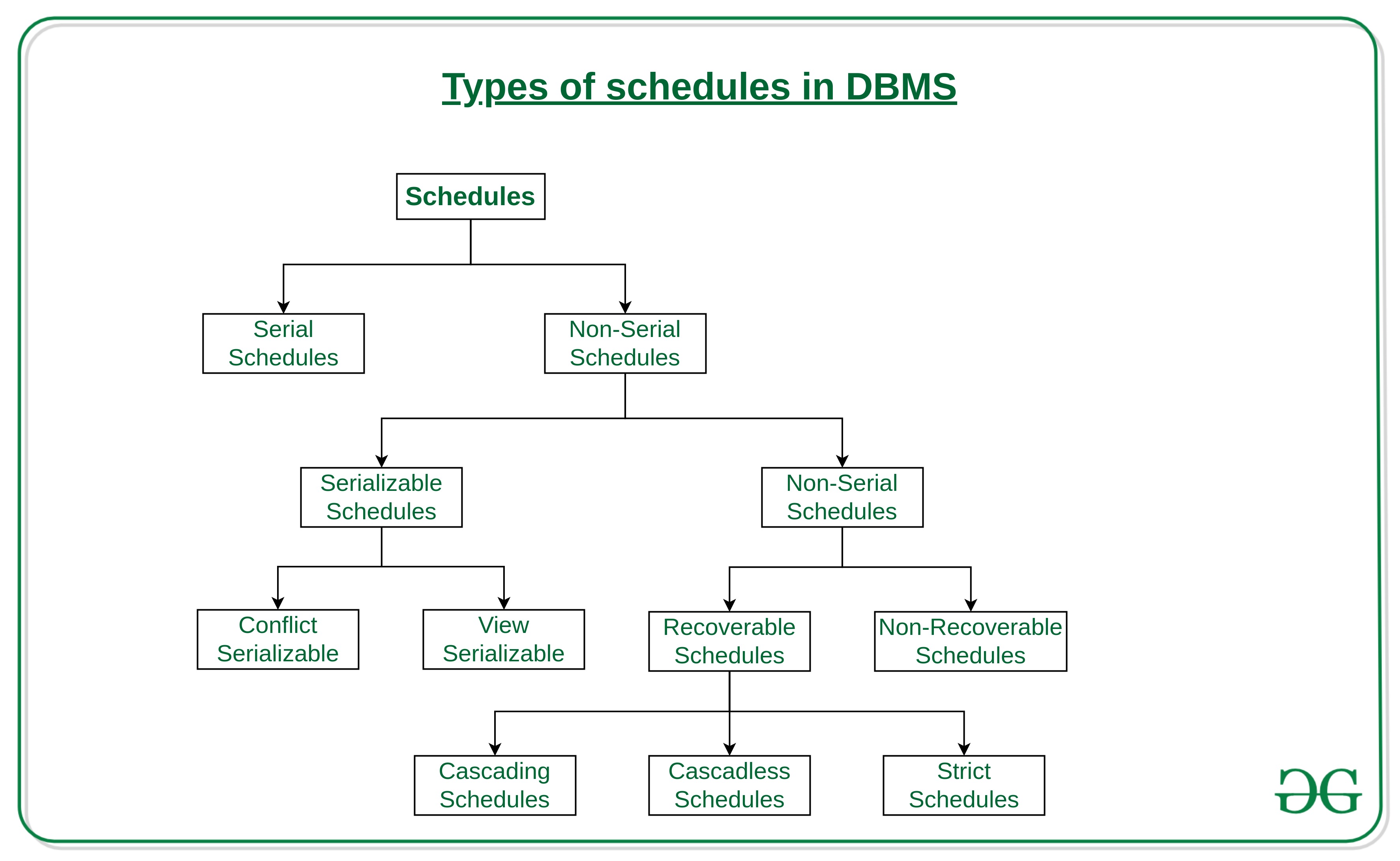
The order in which the operations of multiple transactions appear for execution is called as a schedule.

Serial Schedules –

All the transactions execute serially one after the other.
When one transaction executes, no other transaction is allowed to execute.
Serial schedules are always- Consistent, Recoverable, Cascadeless and Strict.

Non-Serial Schedules –

Multiple transactions execute concurrently.
Operations of all the transactions are inter leaved or mixed with each other.
Non-serial schedules are not always- Consistent, Recoverable, Cascadeless and Strict.

Serializability –

Some non-serial schedules may lead to inconsistency of the database.
Serializability is a concept that helps to identify which non-serial schedules are correct and will maintain the consistency of the database.

Serializable Schedules –

If a given non-serial schedule of ‘n’ transactions is equivalent to some serial schedule of ‘n’ transactions, then it is called as a serializable schedule.
Serializable schedules are always- Consistent, Recoverable, Cascadeless and Strict.

Types of Serializability –

Conflict Serializability

If a given non-serial schedule can be converted into a serial schedule by swapping its non-conflicting operations, then it is called a conflict serializable schedule.

View Serializability

If a given schedule is found to be viewed as equivalent to some serial schedule, then it is called a view serializable schedule.

Non-Serializable Schedules –

A non-serial schedule which is not serializable is called a non-serializable schedule.
A non-serializable schedule is not guaranteed to produce the same effect as produced by some serial schedule on any consistent database.
Non-serializable schedules- may or may not be consistent, may or may not be recoverable.

Irrecoverable Schedules –

If in a schedule,

A transaction performs a dirty read operation from an uncommitted transaction And commits before the transaction from which it has read the value then such a schedule is known as an Irrecoverable Schedule.

Recoverable Schedules –

If in a schedule,

A transaction performs a dirty read operation from an uncommitted transaction And its commit operation is delayed till the uncommitted transaction either commits or roll backs then such a schedule is known as a Recoverable Schedule.

Types of Recoverable Schedules –

Cascading Schedule - If in a schedule, failure of one transaction causes several other dependent transactions to rollback or abort, then such a schedule is called as a Cascading Schedule or Cascading Rollback or Cascading Abort.
Cascadeless Schedule - If in a schedule, a transaction is not allowed to read a data item until the last transaction that has written it is committed or aborted, then such a schedule is called as a Cascadeless Schedule.
Strict Schedule - If in a schedule, a transaction is neither allowed to read nor write a data item until the last transaction that has written it is committed or aborted, then such a schedule is called as a Strict Schedule.

Advantage of Concurrency

Waiting Time
Response Time
Resource Utilization
Efficiency

Problems

Dirty Read Problem
Unrepeatable Read Problem
Phantom Read Problem
Lost Update Problem (Write-Write Conflict)
(blind write)

10. Concurrency Control Technique

Till now we already know how to check weather a schedule will maintain the consitency of DB as not (CS,VS,Recovarability,Cascadless,Strict,etc)
Now will study protocols that guarantee to generate schedule which satisfy these properties speicifically(CS)
for CS we must avoid conflicting instructions we remember three condition of conflicting instruction
Actual Problem is different transaction trying to access data at same time.
How to approach conflict serializability
- Time Stamping Protocol
- Lock based protocol
  - 2PL(Basic,Conservative,Strict,Rigorous)
  - Graph based
- Validation Protocol
Goals (Concurrency,Propeties,time,logic)

Time Stamp Ordering Protocol

Basic Idea of Time Stamping is to decide the order between the transactions before that enters into the system so that in case of conflict during execution we can resolve the conflict using ordering.
The reason we call timestamp not stamp, because for stamping we use the value of system clock as it will always be unique or never respect itself.
Two ideas of time stamping
- Time stamp with transaction - with each transaction ti we associate a time stamp denoted by TS(ti).
- it is the value of the system clock when a transaction enters into the system so if a new transaction tj enters after ti then, TS(ti)< TS(tj) always unique will remain fixed through the execution.
- also determine serializability order if TS(ti) < TS(tj) then system ensure that in the resultant Conflict Serializable Schedule ti will execute fast before tj.
Time stamp with data item - for each data item Q, protocal maintains two time stamp.
- Write time stamp - It is the largest time stamp of any transaction that executed write successfully.
- Read time stamp - It is the largest time stamp of any transaction that executed read successfully.

Ti request for Read (Q)

if TS(ti) < WTS(Q), means Ti needs to read a value of Q that was already overwritten. Hence, request must be rejected & Ti must rollback.
if TS(ti) >= WTS(Q), operation can be allowed and RTS(Q) will be max(RTS(Q),TS(ti))

Ti request for Write (Q)

if TS(ti) < RTS(Q), means value of Q that Ti is producing was needed previously and the system assumed that the value would never be produced hence reject and roll back.
if TS(ti) < WTS(Q), Ti is attempting to write the absolute value of Q reject and Rollback otherwise ok. WTS(Q) = max(WTS(Q),TS(ti))

Properties of Time Stamping Protocol

It ensure conflict serializability.
It ensure view Serializability.
Possibility of dirty read no restriction on commit, irrecoverable schedules and cascading rollbacks are possible.
here Either we allow or reject so no idea of deadblock.
many suffer from starvation. relatively slow.

Thomas Write Rule:

Modifies time stamping protocol to make some improvements and may generate these scheduler that are VS but not CS and provide better concurrency.
it modifies time stamping protocol in absolute write case when Ti request write (Q) if TS(ti) < WTS(Q)
here Ti attempts to write absolute value of Q rather the rolling back Ti, write operator is ignored.

Lock Based Protocol

To achieve consistency isolation is the most important idea, locking is simplest idea to achieve isolation ie. first obtain a lock on a data item performed a desired operation and then unlock it.
to provide better concurrency along with isolation we use different modes of locks.
1. Shared Lock - denoted by lock-S(Q). transaction can perform Read operation, any other transaction can also obtain same lock on same data item at same time.
2. Exclusive Mode - denoted by lock-X(Q) transaction can perform both read/write operations, any other transaction can not obtained either shared/exclusive mode lock.

Properties of Lock Based Protocol

if we do unlocking inconsistency will arise, if we do not unlock then concurrency will be poor.
We require that transaction follow some set of rules for locking and unlocking of data eg. 2PL , graph based.
We say a schedule is legal under a protocoll if it can be generated using the rules of the protocols.
Not Conflict Serializable,irrecoverable, cascading rollbacks.

Two Phase Locking (2PL) Basic

this protocol requires that each transaction in a schedule will be two phased. growing phase and shrinking phase.
In growing phase transaction can only obtain locks but can not release any lock.
In shrinking phase transaction can only release locks but can not obtain any lock.
transaction can perform read/write operation both in growing/shrinking phase.
Ensure (CS,VS) the order of serializability is the order in which transaction reaches lock point.
May generate irrecoverable schedule and cascading rollback.
Do no ensure freedom from deadlock.

Two Phase Lock (Conservative/Static 2PL)

there is no growing phase transaction first will start from lock point.
if all locks are not available then transaction must release the lock acquired so far and wait.
shrinking phase works as usual and transaction can unlock any data item.
here we must have all the knowledge that what data items will be required during execution.
CS,VS indepedent from deadlock.
possiblity of irrecoverable schedule and cascading rollback.

Rigorous 2PL

it is an improvement over 2PL protocol where we try to ensure recoverability and cascade lessons.
Rigorous 2Pl requires that all the locks must be held until transaction commits. ie. there is no shrinking phase in the life of a transaction.
will ensure CS, VS, recoverabillity, cascadelessness.
suffer from deadlock and inefficiency.

Strict 2PL

It is an improvement over Rigorous 2PL.
In the shrinking phase unlocking of exclusive locks are not allowed but unlocking of shared locks can be done.
all the properties are same as that of rigourous 2PL, but it provide better concurrency.

Graph Based Protocol

if we wish to develop lock based protocol that are not based on 2PL, we need additional info that how each transaction will access the data.
there are various model that can give additional information each differing in the amount of info provided.
one idea is to have prior knowledge about the order in which the database items will be accessed.
we impose partial ordering => on set all data items D={d1,d2,d3,….dn} if di->dj, then any transaction occcuring both di and dj, must access di before dj.
Partial Ordering may be bacause logical or physical organization or only because of concurrency control.
After PO set of all data items D will know be viewed as directed acyclic graph called database graph.
For sake of simplicity, we follow two restrictions
- will study graph that are rooted tree.
- will use only exclusive mode locks.

Tree Protocol

Each transaction Ti can lock a data item Q with following rules:
1. First lock by Ti may be on any data item.
2. Subsequently a data item Q can be locked by Ti only if the parent of Q is currently locked by Ti.
3. Data item may be unlocked at any time.
4. Data item Q that has been locked and unlocked by Ti can not subsequently be relocked by Ti.

Properties of Tree Protocol

All schedules that are legal under the tree protocol are CS and VS.
Tree protocol ensure freedom from deadlock.
Tree protocol do not ensure Recoverability and Cascadlessness.
Early unlocking is possible which lead shortest waiting time on increase concurrency.
A transaction may have to take data items that it does not access lead to overhead waiting time and decrease in concurrency.
Transaction must know exactly what data item are to be accessed.
Recoverability and Cascadlessness can be provided by not unlocking before commit.

B Trees

At every level , we have Key and Data Pointer and data pointer points to either block or record.

Properties of B-Trees:

Root of B-tree can have children between 2 and P, where P is Order of tree.

Order of tree – Maximum number of children a node can have. Internal node can have children between ⌈ P/2 ⌉ and P Internal node can have keys between ⌈ P/2 ⌉ – 1 and P-1

B+ Trees

In B+ trees, the structure of leaf and non-leaf are different, so their order is.
Order of non-leaf will be higher as compared to leaf nodes.
Searching time will be less in B+ trees, since it doesn’t have record pointers in non-leaf because of which depth will decrease.

Deadlock handling

A system is in deadlock state if there exists a set of transaction such that every transaction in the set is waiting for another transaction in the set.
if there exists a set of waiting transaction T0,T1…..Tn-1 such that T0->T1, T1->T2 ….. Tn-1->T0 so none transaction can progress in such situation.
system must have a proper methods to dead with deadlocks otherwise
- In real time system it may lead to life and money.
- will reduce resource utilization and increase inefficiency.
there are two principle for dealing with deadlock problem.
- Prevention - which ensure that system will never enter a deadlock state.
- Detection and Recovery = allow system to enter into deadlock, then try to recover

Deadlock Prevention

To ensure no hold & wait, each transaction locks all the data item before it begins execution. eg C-2PL.
To ensure no cyclic wait, impose an ordering og all data item, and requires that a transaction look data item, only in the sequence consistent with ordering eg.tree protocol.
- it is difficult to predict what data items are required.
- data item utilization will be low.
- ordering of data item may be difficult or time taking to follow.
wait and Die (Non-premptive)
wound and wait (Premptive)
lock-timeouts

8. SQL

Query Languages

After Designing of database. ie. ER Diagram design then converting it into relational model followed by normalization and indexing now task is how to store, retrieve and modify data in database.
Query Languages - Languages in which user request some information from databse.
Procedural Query Language - Here user instruct the system to perform sequence of operations in order to produre desired result. User tell what data to be retrieved and how to be retrieved.
Non-Procedural Query Language - Here user descrive the desired information without giving the specific procedure for obtaining that information.

Relational Algebra

In practice we use RDBMS(Practical Implementation of relational model)
SQL is used to write query on it.
So Relational Model is a conceptual/theoritical framework and RDBMS is it implementaion.
Relational Algebra(Procedural) and Relational Calculus (non-procedural) are mathematical system are query language used on Relational model.

Query Language - Procedural and Non-Procedural Procedural - Relational Algebra Non-Procedural - Relational Calculus Relational Algebra and Relational Calculus = SQL


Relational Model	RDBMS
RA, RC	SQL
Algo	Code
Conceptual	Reality
Theoretical	Practical

Relational Algebra

Relational Algebra is one of the two formal query language associated with relational model.
Like any other mathematical system is defines a number of operators and use relational (tables) as operands.
Every operator in relation algebra take one or two relations are input argument and generate a single relation as a result without a name.
RA do not consider duplicacy as it’s based on set theory.
In each query we describes a step by step procedure for computing the desired result so procedural QL.
No use of English Keywords.

Basic/Fundamental Operators	Derived Operators
Select ( σ )	Natural Join ( ⋈ )
Project ( π )	Intersection ( ∩ )
Union ( ∪ )	Division ( ÷ )
Set Diffrence ( - )
Cartesian Product ( X )
Rename ( ρ )

Relational Algebra

Relational Algebra is a procedural query language which takes a relation as an input and generates a relation as an output.

Basic Operator	Semantic
σ(Selection)	Select rows based on given condition
∏(Projection)	Project some columns
X (Cross Product)	Cross product of relations, returns m*n rows where m and n are number of rows in R1 and R2 respectively.
U (Union)	Return those tuples which are either in R1 or in R2. Max no. of rows returned = m+n and Min no. of rows returned = max(m,n
−(Minus)	R1-R2 returns those tuples which are in R1 but not in R2. Max no. of rows returned = m and Min no. of rows returned = m-n
ρ(Rename)	Renaming a relation to another relation

Extended Operator	Semantic
∩ (Intersection)	Returns those tuples which are in both R1 and R2. Max no. of rows returned = min(m,n) and Min no. of rows returned = 0
⋈c(Conditional Join)	Selection from two or more tables based on some condition (Cross product followed by selection)
⋈(Equi Join)	It is a special case of conditional join when only equality conditions are applied between attributes
⋈(Natural Join)	In natural join, equality conditions on common attributes hold and duplicate attributes are removed by default.
Note: Natural Join is equivalent to cross product if two relations have no attribute in common and natural join of a relation R with itself will return R only
⟕(Left Outer Join)	When applying join on two relations R and S, some tuples of R or S do not appear in the result set which does not satisfy the join conditions. But Left Outer Joins gives all tuples of R in the result set. The tuples of R which do not satisfy the join condition will have values as NULL for attributes of S
⟖(Right Outer Join)	When applying join on two relations R and S, some tuples of R or S do not appear in the result set which does not satisfy the join conditions. But Right Outer Joins gives all tuples of S in the result set. The tuples of S which do not satisfy the join condition will have values as NULL for attributes of R
⟗(Full Outer Join)	When applying join on two relations R and S, some tuples of R or S do not appear in the result set which does not satisfy the join conditions. But Full Outer Joins gives all tuples of S and all tuples of R in the result set. The tuples of S which do not satisfy the join condition will have values as NULL for attributes of R and vice versa.
/(Division Operator)	Division operator A/B will return those tuples in A which are associated with every tuple of B. Note: Attributes of B should be a proper subset of attributes of A. The attributes in A/B will be Attributes of A- Attribute of B.

SELECT Operator ( σ )

Select is a unary operator so can take only one table at a time.
It is a fundamental Operator.
Main idea of select is to find these tuples/rows in a relation which satisfied given condition.
Syntax => σ condition/predicate^(table name)
It is same function as of where clause in SQL.
min number of selected is 0.
max number of selected is all the tuples.

Project Operator ( π )

Unary Operator, take one table at a time.
Fundamental Operator
Main idea of project is select desired column
Syntax π column name ^ (table name)
It works as select clause of SQL

Union Intersection and set difference

Cross Product and Cartesian Product

Binary Operator, takes two tables at a time.
Funadamental Operator
Allow us to combine information between two tables.
R1 = m, R2 = n, R1xR2 = mn
R1(A,B,C), R2(C,D,F), R1xR2(A,B,C,D,F) no.of column

Introduction to SQL

Number of query languages are in use/around 50 are popular, both commercially and research.
The most popular and widely accepted query language is SQL (Structures Query Language)
SQL is domain specific not general purpose used in design and management of data held in RDBMS.
Can do much more than just query a database can define structure of data, modify data in data base specify securiity constraints and number of other tasks.
Based on relational algebra and tuple relational calculus.
IBM developed original version of SQL called SEQUEL in Project R in early 1970
Name later changed to SQL becuase of trademark issues.
In 1986, American National Standard Institute (ANSI) and ISO published SQL Standard called SQL-86
Next version, 1989, 1992, 1999, 2003, 2006, 2008, 2011 and most recently 2016.
Data Definition Language - DDL is short name of Data Definition Language, which deals with database schemas and descriptions, of how the data should reside in the database.
- Integrity - Provide commands for integrity constraints on the data stored in DB. eg. Primary key cannot be null, foreign key reference.
- View definition - command for defining views. eg. sorting the result according to same attribute.
- Authorization - commands for access right. eg. read only, R/W grants etc.
- ex.
- CREATE - to create a database and its objects like (table, index, views, store procedure, function, and triggers)
- ALTER - alters the structure of the existing database
- DROP - delete objects from the database
- TRUNCATE - remove all records from a table, including all spaces allocated for the records are removed
- RENAME - rename an object
Data Manipulation Language - DML is short name of Data Manipulation Language which deals with data manipulation and includes most common SQL statements such SELECT, INSERT, UPDATE, DELETE, etc., and it is used to store, modify, retrieve, delete and update data in a database.
- Transaction Control - SQL includes commands for specifying the beginning and ending of transactions. eg. commit, rollback, squ points, etc.
- Embedded SQL and Dynamic SQL - how SQL statemnet can be embedded with in general purpose programming language such as C, C++, Java, etc.
- ex
- SELECT - retrieve data from a database
- INSERT - insert data into a table
- UPDATE - updates existing data within a table
- DELETE - Delete all records from a database table
- MERGE - UPSERT operation (insert or update)

Data Control Language

DCL is short name of Data Control Language which includes commands such as GRANT and mostly concerned with rights, permissions and other controls of the database system.
- GRANT - allow users access privileges to the database
- REVOKE - withdraw users access privileges given by using the GRANT command

Transaction Control Language

TCL is short name of Transaction Control Language which deals with a transaction within a database.
- COMMIT - commits a Transaction
- ROLLBACK - rollback a transaction in case of any error occurs
- SAVEPOINT - to roll back the transaction making points within groups

SQL:

SQL is a standard language for storing, manipulating and retrieving data in databases.

Data Retrieval

for data retrival in SQL i/p and o/p both are relations.
no. of relation i/p to query will be at least are but o/p will always be a singel relation without any name unless specified.
Basic structure of SQL query consist of these clauses. (SELECT FROM WHERE)
It should noted that SELECT and FROM mandatory and if not required, then not necessary to write WHERE
SQL in general is not case sensitive
SQL allows duplication in a i/p relation as well as in the result of SQL expression.

SELECT Clause

is used to pick columns required in result of the query out of all columns in i/p relation.
order in which column are represented in the select closure will be same in which column will appear in the result.
if all columns are required then * can be used.
may also contains arithmetic expression involving operators like +, -, /, * etc however it does not change to the database.
DISTINCT keyword to remove duplicacy

SELECT with WHERE

where clause in SQL is used to specify conditions/predicates.
where closure can have expression involving comparisons operator <,<=,>,>=,=,<> etc.
SQL allows use of logical connectives and, or, not etc.
allows ‘between’ comparision operator to simplify where clause which specify >= to some value and <= to some other value.
similarly can use ‘not between’.

Set Operations

SQL provides set operations Union, Intersect, except/minus/set difference which correspons to the mathematical set operations.
Here union, intersect, minus automatically eliminates duplicate tuple.
if we want to retain duplicate tuple we write [all’ after operators.
set operations are only applicable between two relations if they are compatible ie. having same number of columns with correspondingly same domain.

Queries on multiple relations(Cartesian Product)

so for we have worked on simple query requires only one relation.
Queries often need more than one realtion for information and to do that are simole idea is cartesian product.
CP combine two relation into one by Concatenation each tuple of first relation with every possible tuple of second relation.
CP is commutative in nature so order does not matter
if same attribute name appears as in both relation, we prefix the name of relation from which attribute originally comes.

Queries on multiple relations (Natural Join)

Basically natural join work same as cartesian product but consider only three pair of tuples with the same value on these attribute that appear in the schemas of both relation.
Notice that common attribute comes only once and prev is also not required as we allow only same value
commutative in nature.
may lead to data loss if attributes to be match have different names,or some values occur only in one table.

Join/Inner Join

is an operation which works same as cartesian product if used alone.
but if join is used with keyword using it provides additional functionality.
provides ability to explicitly share column which must be used by join for comparision and removal of redundant tuples.
if there are more than one column common between two tables but we do not want each of them to be considered, then we specify which are to be considred by using operator.

Join with on

In SQL join with ‘on’ allows us to use a general pedicate over the relations being joined.
this predicate is written like a where predicate except for the use of the keyowrd on rather than where
like CP here we must specify which attribute must be matched.
more powerful as predicate of where can also be written with on
on condition can express any SQL predicate
it imoproves the readability of the query.
in case of outer join on condition behave differently from where

Outer join

One problem with natural join is only those value that appear in both relation will manage to reach find table.
but if some data is explicitly in table one as table two then that will be lost.
there are three from of outer join
- left outer join (left join)
- right outer join (right join)
- full outer join (full join/ complete join)

Rename Operation (as)

SQL aliases are used to give table or column of a table or column of a table a temporary name.
Aliases only exists for the duration of the query.
Uses as clause can appear both in select and from clause.
often used to name more readable meaning full as smaller
used for comparing a table with it self.
new temporary name of table know as table aliases/corelation varibles/tuple variable.
Just creates a new copy but do not change anything in database.

String Operations

SQL specifies strings by enclosing them in single quotes ‘Knowledge Gate’
Equality operation on string may or may not be case sensitive. eg. most of the Db system are case sensitive but MySQL and SQL server are not we can change the behaviour in settings.
Number of operations are available on string such as conatenation substrings finding length of strings converting string to uppercase or lowercase, etc
exact set of operations may change from system to system.
pattern matching can be performed on a string using ‘like’ operator.
two special character -> Percent(): match any substring -> underscore(): matches with any character
Pattern matching is case sensitive
if single quote is part of a string, it must be specified by two singel quote
for pattern which includs pattern we use escape character just before the special character.

Ordering the display of tuple

SQL offer the user some control over the order in which tuples in a relation are displayed
OrderBy clause causes the tuple in the result of a query to appear in sorted order
By default order by clause lists items in ascening order we may specify asc for ascending order and desc for descending order.
ordering can be performed on multiple attribute ie. if there is a tie on the first attribute we sorted according to second attribute.

SELECT:

The SELECT statement is used to select data from a database.

Syntax -
- SELECT column1, column2, … FROM table_name;
- Here, column1, column2, … are the field names of the table you want to select data from.
- If you want to select all the fields available in the table, use the following syntax:
- SELECT * FROM table_name;
Ex –
- SELECT CustomerName, City FROM Customers;

SELECT DISTINCT:

The SELECT DISTINCT statement is used to return only distinct (different) values.

Syntax –
- SELECT DISTINCT column1, column2, … FROM table_name;
Ex –
- SELECT DISTINCT Country FROM Customers;

WHERE:

The WHERE clause is used to filter records.

Syntax –
- SELECT column1, column2, … FROM table_name WHERE condition;
Ex –
- SELECT * FROM Customers WHERE Country=’Mexico’;

Operators

Operator	Description
=	Equal
>	Greater than
<	Less than
>=	Greater than or equal
<=	Less than or equal
<>	Not equal. Note: In some versions of SQL this operator may be written as !=

AND, OR and NOT:

The WHERE clause can be combined with AND, OR, and NOT operators.
The AND and OR operators are used to filter records based on more than one condition:
- The AND operator displays a record if all the conditions separated by AND are TRUE.
- The OR operator displays a record if any of the conditions separated by OR is TRUE.
The NOT operator displays a record if the condition(s) is NOT TRUE.
Syntax –
- SELECT column1, column2, … FROM table*name WHERE condition1 AND condition2 AND condition3 …;
- SELECT column1, column2, … FROM table_name WHERE condition1 OR condition2 OR condition3 …;
- SELECT column1, column2, … FROM table_name WHERE NOT condition;
Ex –
- SELECT * FROM Customers WHERE Country=’Germany’ AND City=’Berlin’;
- SELECT * FROM Customers WHERE Country=’Germany’ AND (City=’Berlin’ OR City=’München’);

ORDER BY:

The ORDER BY keyword is used to sort the result-set in ascending or descending order.
The ORDER BY keyword sorts the records in ascending order by default. To sort the records in descending order, use the DESC keyword.
Syntax –
- SELECT column1, column2, … FROM table*name ORDER BY column1, column2, … ASC|DESC;
Ex –
- SELECT * FROM Customers ORDER BY Country;
- SELECT * FROM Customers ORDER BY Country ASC, CustomerName DESC;

INSERT INTO:

The INSERT INTO statement is used to insert new records in a table.

Syntax –
- INSERT INTO table_name (column1, column2, column3, …) VALUES (value1, value2, value3, …);
- INSERT INTO table_name VALUES (value1, value2, value3, …);

*In the second syntax, make sure the order of the values is in the same order as the columns in the table.

Ex –
- INSERT INTO Customers (CustomerName, ContactName, Address, City, PostalCode, Country) VALUES (‘Cardinal’, ‘Tom B. Erichsen’, ‘Skagen 21’, ‘Stavanger’, ‘4006’, ‘Norway’);

NULL Value:

It is not possible to test for NULL values with comparison operators, such as =, <, or <>. We will have to use the IS NULL and IS NOT NULL operators instead.
Syntax –
- SELECT column*names FROM table_name WHERE column_name IS NULL;
- SELECT column_names FROM table_name WHERE column_name IS NOT NULL;
Ex –
- SELECT CustomerName, ContactName, Address FROM Customers WHERE Address IS NULL;

UPDATE:

The UPDATE statement is used to modify the existing records in a table.

Syntax –
- UPDATE table_name SET column1 = value1, column2 = value2, … WHERE condition;
Ex –
- UPDATE Customers SET ContactName = ‘Alfred Schmidt’, City= ‘Frankfurt’ WHERE CustomerID = 1;

DELETE:

The DELETE statement is used to delete existing records in a table.

Syntax –
DELETE FROM table_name WHERE condition;
DELETE FROM table_name;

In 2ndsyntax, all rows are deleted. The table structure, attributes, and indexes will be intact

Ex –
- DELETE FROM Customers WHERE CustomerName=’Alfreds Futterkiste’;

SELECT TOP:

The SELECT TOP clause is used to specify the number of records to return.

Syntax –
- SELECT TOP number|percent column_name(s) FROM table_name WHERE condition;
- SELECT column_name(s) FROM table_name WHERE condition LIMIT number;
- SELECT column_name(s) FROM table_name ORDER BY column_name(s) FETCH FIRST number ROWS ONLY;
- SELECT column_name(s) FROM table_name WHERE ROWNUM <= number;

*In case the interviewer asks other than the TOP, rest are also correct. (Diff. DB Systems)

Ex –
- SELECT TOP 3 * FROM Customers;
- SELECT * FROM Customers LIMIT 3;
- SELECT * FROM Customers FETCH FIRST 3 ROWS ONLY;

Aggregate Functions:

MIN():

The MIN() function returns the smallest value of the selected column.

Syntax –
- SELECT MIN(column*name) FROM table_name WHERE condition;
Ex –
- SELECT MIN(Price) AS SmallestPrice FROM Products;

MAX():

The MAX() function returns the largest value of the selected column.

Syntax –
- SELECT MAX(column_name) FROM table_name WHERE condition;
Ex –
- SELECT MAX(Price) AS LargestPrice FROM Products;

COUNT():

The COUNT() function returns the number of rows that matches a specified criterion.

Syntax –
- SELECT COUNT(column_name) FROM table_name WHERE condition;
Ex –
- SELECT COUNT(ProductID) FROM Products;

AVG():

The AVG() function returns the average value of a numeric column.

Syntax –
- SELECT AVG(column_name) FROM table_name WHERE condition;
Ex –
- SELECT AVG(Price) FROM Products;

SUM():

The SUM() function returns the total sum of a numeric column.

Syntax –
- SELECT SUM(column_name) FROM table_name WHERE condition;
Ex –
- SELECT SUM(Quantity) FROM OrderDetails;

LIKE Operator:

The LIKE operator is used in a WHERE clause to search for a specified pattern in a column. There are two wildcards often used in conjunction with the LIKE operator:

The percent sign (%) represents zero, one, or multiple characters
The underscore sign (*) represents one, single character
Syntax –
- SELECT column1, column2, … FROM table_name WHERE columnN LIKE pattern;

LIKE Operator	Description
WHERE CustomerName LIKE ‘a%’	Finds any values that start with “a”
WHERE CustomerName LIKE ‘%a’	Finds any values that end with “a”
WHERE CustomerName LIKE ‘%or%’	Finds any values that have “or” in any position

WHERE CustomerName LIKE ‘_r%’	Finds any values that have “r” in the second position
WHERE CustomerName LIKE ‘a_%’	Finds any values that start with “a” and are at least 2 characters in length
WHERE CustomerName LIKE ‘a__%’	Finds any values that start with “a” and are at least 3 characters in length
WHERE ContactName LIKE ‘a%o’	Finds any values that start with “a” and ends with “o”

IN:

The IN operator allows you to specify multiple values in a WHERE clause. The IN operator is a shorthand for multiple OR conditions.

Syntax –
- SELECT column*name(s) FROM table_name WHERE column_name IN (value1, value2, …);
- SELECT column_name(s) FROM table_name WHERE column_name IN (SELECT STATEMENT);
Ex –
- SELECT * FROM Customers WHERE Country IN (‘Germany’, ‘France’, ‘UK’);
- SELECT _ FROM Customers WHERE Country IN (SELECT Country FROM Suppliers);

BETWEEN:

The BETWEEN operator selects values within a given range. The values can be numbers, text, or dates. The BETWEEN operator is inclusive: begin and end values are included.

Syntax –
- SELECT column_name(s) FROM table_name WHERE column_name BETWEEN value1 AND value2;
Ex –
- SELECT * FROM Products WHERE Price BETWEEN 10 AND 20;

Joins:

A JOIN clause is used to combine rows from two or more tables, based on a related column between them.

INNER JOIN:

The INNER JOIN keyword selects records that have matching values in both tables.

Syntax –
- SELECT column_name(s) FROM table1 INNER JOIN table2 ON table1.column_name = table2.column_name;
Ex –
- SELECT Orders.OrderID, Customers.CustomerName FROM Orders INNER JOIN Customers ON Orders.CustomerID = Customers.CustomerID;

LEFT (OUTER) JOIN:

The LEFT JOIN keyword returns all records from the left table (table1), and the matching records from the right table (table2). The result is 0 records from the right side, if there is no match.

Syntax –
- SELECT column_name(s) FROM table1 LEFT JOIN table2 ON table1.column_name = table2.column_name;
Ex –
- SELECT Customers.CustomerName, Orders.OrderID FROM Customers LEFT JOIN Orders ON Customers.CustomerID = Orders.CustomerID ORDER BY Customers.CustomerName;

RIGHT (OUTER) JOIN:

The RIGHT JOIN keyword returns all records from the right table (table2), and the matching records from the left table (table1). The result is 0 records from the left side, if there is no match.

Syntax –
- SELECT column_name(s) FROM table1 RIGHT JOIN table2 ON table1.column_name = table2.column_name;
Ex –
- SELECT Orders.OrderID, Employees.LastName, Employees.FirstName FROM Orders RIGHT JOIN Employees ON Orders.EmployeeID = Employees.EmployeeID ORDER BY Orders.OrderID;

FULL (OUTER) JOIN:

The FULL OUTER JOIN keyword returns all records when there is a match in left (table1) or right (table2) table records.

Syntax:
- SELECT column_name(s) FROM table1 FULL OUTER JOIN table2 ON table1.column_name = table2.column_name WHERE condition;
Ex –
- SELECT Customers.CustomerName, Orders.OrderID FROM Customers FULL OUTER JOIN Orders ON Customers.CustomerID=Orders.CustomerID ORDER BY Customers.CustomerName;

UNION:

The UNION operator is used to combine the result-set of two or more SELECT statements.

Every SELECT statement within UNION must have the same number of columns - The columns must also have similar data types
The columns in every SELECT statement must also be in the same order The UNION operator selects only distinct values by default. To allow duplicate values, use UNION ALL
Syntax –
- SELECT column_name(s) FROM table1 UNION SELECT column_name(s) FROM table2;
- SELECT column_name(s) FROM table1 UNION ALL SELECT column_name(s) FROM table2;
Ex –
- SELECT City FROM Customers UNION SELECT City FROM Suppliers ORDER BY City;

GROUP BY:

The GROUP BY statement groups rows that have the same values into summary rows, like “find the number of customers in each country”. The GROUP BY statement is often used with aggregate functions (COUNT(), MAX(), MIN(), SUM(), AVG()) to group the result-set by one or more columns.

Syntax –
- SELECT column_name(s) FROM table_name WHERE condition GROUP BY column_name(s) ORDER BY column_name(s);
Ex –
- SELECT COUNT(CustomerID), Country FROM Customers GROUP BY Country ORDER BY COUNT(CustomerID) DESC;

HAVING:

The HAVING clause was added to SQL because the WHERE keyword cannot be used with aggregate functions. *WHERE is given priority over HAVING.

Syntax –
- SELECT column_name(s) FROM table_name WHERE condition GROUP BY column_name(s) HAVING condition ORDER BY column_name(s);
Ex –
- SELECT COUNT(CustomerID), Country FROM Customers GROUP BY Country HAVING COUNT(CustomerID) > 5;

CREATE DATABASE:

The CREATE DATABASE statement is used to create a new SQL database.

Syntax –
- CREATE DATABASE databasename;

DROP DATABASE:

The DROP DATABASE statement is used to drop an existing SQL database.

Syntax –
- DROP DATABASE databasename;

CREATE TABLE:

The CREATE TABLE statement is used to create a new table in a database.

Syntax –
- CREATE TABLE table_name ( column1 datatype, column2 datatype, column3 datatype, …. );

DROP TABLE:

The DROP TABLE statement is used to drop an existing table in a database.

Syntax –
- DROP TABLE table_name;

TRUNCATE TABLE:

The TRUNCATE TABLE statement is used to delete the data inside a table, but not the table itself.

Syntax –
- TRUNCATE TABLE table_name;

ALTER TABLE:

The ALTER TABLE statement is used to add, delete, or modify columns in an existing table. The ALTER TABLE statement is also used to add and drop various constraints on an existing table.

Syntax –
- ALTER TABLE table_name ADD column_name datatype;
- ALTER TABLE table_name DROP COLUMN column_name;
- ALTER TABLE table_name MODIFY COLUMN column_name datatype;
Ex –
- ALTER TABLE Customers ADD Email varchar(255);
- ALTER TABLE Customers DROP COLUMN Email;
- ALTER TABLE Persons ALTER COLUMN DateOfBirth year;

DBMS

Note - This notes are made from videos of Sanchit Jain Youtube (Knowledge Gate). I will really suggest to watch those videos because he explained all these really well. I can guarantee that you will not get bored at any point.

Basic Fundamentals

Difference between Data, Information, Database

Disadvantage of File System

OLAP VS OLTP

1. Entity Relationship Diagram

Introduction and Basics

Entity, Entity Sets and its types

ER Diagram and Relationship Model

Attributes

Types of Attributes

Relationship in a ER Diagram

Degree of a relationship in a ER diagram

Cardinality Ratio and Mapping Cardinalities

Constraints:

Keys:

Types of Keys:

Participation Constraints

3. Functional Dependency

Functional Dependencies

Types of Functional dependency

Closure of Attribute Set

Armstrong’s Axiom/Rule

Primary Rules (RAT)

Secondary Rules

Equivalency of Functional Dependency

Canonical Cover, Minimal Set, Irreducible set of FD

6. Decomposition of a Relation:

Properties of Decomposition:

Types of Decomposition:

5. Normalization

Why need of Normalization

Idea

Result

Disadvantages

Insertion anomalies

Deletion anomalies

Updation/Modification Anomalies

Normalization

Normal Forms

1NF First Noraml Form

2NF Second Normal Form

Prime Non-Prime Attribute

Partial Dependency

3NF Third Normal Form

Transitive Dependency:

BCNF

7. Indexing and Physical Structure (B, B+ Tree)

File Structure

Indexing

Types of Indexing

Primary Indexing

Clustered Indexing

Secondary Indexing

9. Transaction and Concurrency Control

What is Transaction

Operations in Transaction:

Transaction ACID properties

Transaction States

Schedules:

Serial Schedules –

Non-Serial Schedules –

Serializability –

Serializable Schedules –

Types of Serializability –

Conflict Serializability

View Serializability

Non-Serializable Schedules –

Irrecoverable Schedules –

Recoverable Schedules –

Types of Recoverable Schedules –

Advantage of Concurrency

Problems

10. Concurrency Control Technique

Time Stamp Ordering Protocol

Ti request for Read (Q)

Ti request for Write (Q)

Properties of Time Stamping Protocol

Thomas Write Rule: